Start Here#
PyAutoGalaxy AI Assistant#
The PyAutoGalaxy AI Assistant supports conversation agents such as ChatGPT and coding agents such as Claude Code and Codex. You can get started simply by asking it a question about galaxy structure or describing the task you would like to perform with PyAutoGalaxy. See the assistant for its full scope and instructions.
Human-Readable Overview#
PyAutoGalaxy is software for analysing the morphologies and structures of galaxies:
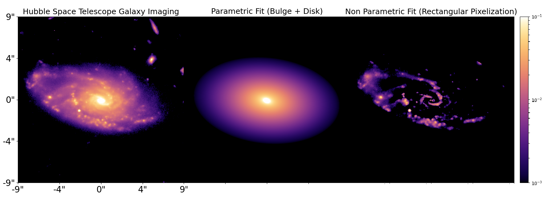
PyAutoGalaxy has three core aims:
Big Data: Scaling automated Sérsic fitting to extremely large datasets, accelerated with JAX on GPUs and using tools like an SQL database to **build a scalable scientific workflow**.
Model Complexity: Fitting complex galaxy morphology models (e.g. Multi Gaussian Expansion, Shapelets, Ellipse Fitting, Irregular Meshes) that go beyond just simple Sérsic fitting.
Data Variety: Support for many data types (e.g. CCD imaging, interferometry, multi-band imaging) which can be fitted independently or simultaneously.
This overview gives an overview of PyAutoGalaxy’s API, core features and details of the autogalaxy_workspace.
Imports#
Lets first import autogalaxy, its plotting module and the other libraries we’ll need.
You’ll see these imports in the majority of workspace examples.
import autogalaxy as ag
import autogalaxy.plot as aplt

import matplotlib.pyplot as plt
from os import path
Lets illustrate a simple galaxy structure calculations creating an an image of a galaxy using a light profile.
Grid#
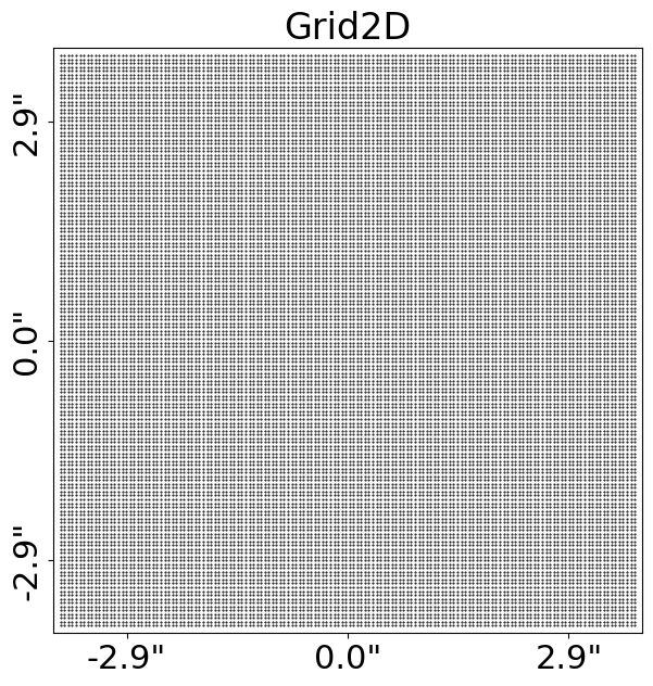
The emission of light from a galaxy is described using the Grid2D data structure, which is two-dimensional
Cartesian grids of (y,x) coordinates where the light profile of the galaxy is evaluated on the grid.
We make and plot a uniform Cartesian grid:
grid = ag.Grid2D.uniform(
    shape_native=(150, 150),  # The [pixels x pixels] shape of the grid in 2D.
    pixel_scales=0.05,  # The pixel-scale describes the conversion from pixel units to arc-seconds.
)

aplt.plot_grid(grid=grid, title="Uniform Grid")
The Grid2D looks like this:
Light Profiles#
Our aim is to create an image of the morphological structures that make up a galaxy.
This uses analytic functions representing a galaxy’s light, referred to as LightProfile objects.
The most common light profile in Astronomy is the elliptical Sersic, which we create an instance of below:
sersic_light_profile = ag.lp.Sersic(
    centre=(0.0, 0.0),  # The light profile centre [units of arc-seconds].
    ell_comps=(
        0.2,
        0.1,
    ),  # The light profile elliptical components [can be converted to axis-ratio and position angle].
    intensity=0.005,  # The overall intensity normalisation [units arbitrary and are matched to the data].
    effective_radius=2.0,  # The effective radius containing half the profile's total luminosity [units of arc-seconds].
    sersic_index=4.0,  # Describes the profile's shape [higher value -> more concentrated profile].
)
By passing the light profile the grid, we evaluate the light emitted at every (y,x) coordinate and therefore create
an image of the Sersic light profile.
image = sersic_light_profile.image_2d_from(grid=grid)
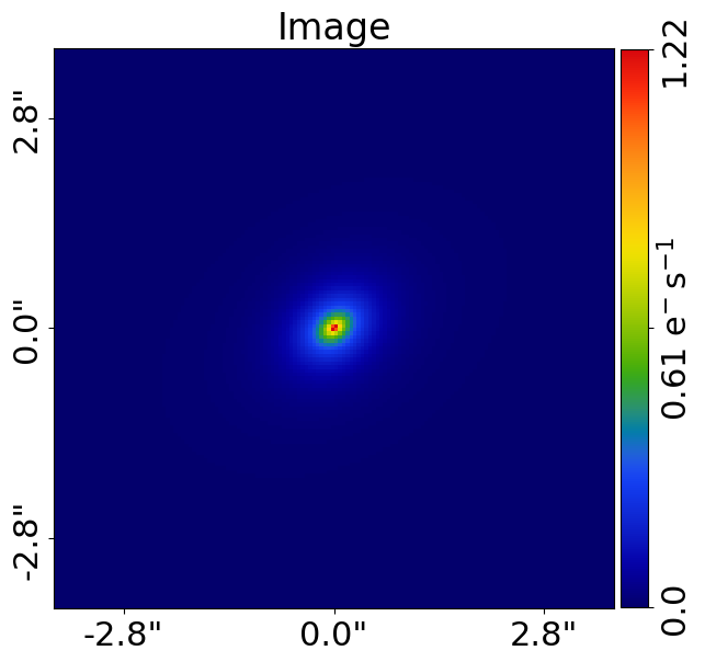
Plotting#
In-built plotting methods are provided for plotting objects and their properties, like the image of a light profile we just created.
By using aplt.plot_array to plot the light profile’s image, the figure is improved.
Its axis units are scaled to arc-seconds, a color-bar is added, descriptive labels are included, etc.
The plot module is highly customizable and designed to make it straight forward to create clean and informative figures for fits to large datasets.
aplt.plot_array(array=sersic_light_profile.image_2d_from(grid=grid), title="Sersic Light Profile Image")
The light profile appears as follows:
Galaxy#
A Galaxy object is a collection of light profiles at a specific redshift.
This object is highly extensible and is what ultimately allows us to fit complex models to galaxy images.
Below, we combine the Sersic light profile above with an Exponential light profile to create a galaxy containing both a bulge and disk component.
exponential_light_profile = ag.lp.Exponential(
    centre=(0.0, 0.0), ell_comps=(0.1, 0.0), intensity=0.1, effective_radius=0.5
)

galaxy = ag.Galaxy(
    redshift=0.5, bulge=sersic_light_profile, disk=exponential_light_profile
)
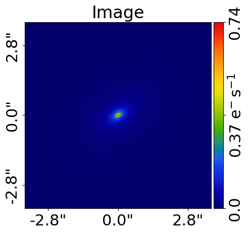
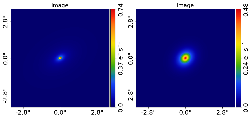
We can plot the image of the galaxy, which is the sum of its bulge and disk light profiles:
aplt.plot_array(array=galaxy.image_2d_from(grid=grid), title="Galaxy Image")
The galaxy, with both a bulge and disk, appears as follows:
The individual light profiles of the galaxy can be plotted on a subplot:
aplt.subplot_galaxy_light_profiles(galaxy=galaxy, grid=grid)
The light profiles appear as follows:
Galaxies#
The Galaxies object is a collection of galaxies at the same redshift.
In a moment, we will see it is integral to the model-fitting API.
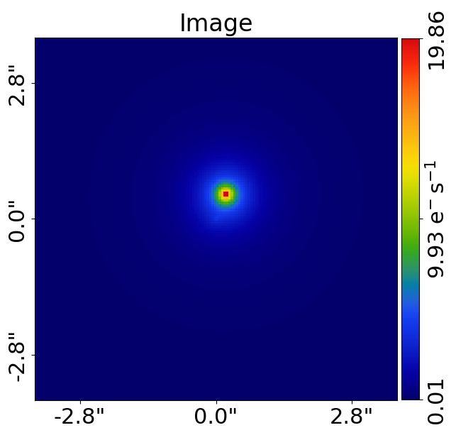
For now, lets use it to create an image of a pair of merging galaxies, noting that a more concise API for creating
the galaxy is used below where the Sersic is passed directly to the Galaxy object.
galaxy_1 = ag.Galaxy(
    redshift=0.5,
    bulge=ag.lp.Sersic(
        centre=(0.5, 0.2), intensity=1.0, effective_radius=1.0, sersic_index=2.0
    ),
)

galaxies = ag.Galaxies(
    galaxies=[galaxy, galaxy_1],
)

aplt.plot_array(array=galaxies.image_2d_from(grid=grid), title="Galaxies Image")
Units#
The units used throughout the galaxy structure literature vary, therefore lets quickly describe the units used in PyAutoGalaxy.
Most distance quantities, like an effective_radius are quantities in terms of angles, which are defined in units
of arc-seconds. To convert these to physical units (e.g. kiloparsecs), we use the redshift of the galaxy and an
input cosmology. A run through of all normal unit conversions is given in guides in the workspace outlined below.
The use of angles in arc-seconds has an important property, it means that calculations are independent of the galaxy’s redshifts and the input cosmology. This has a number of benefits, for example it makes it straight forward to compare the properties of different galaxies even when the redshifts of the galaxies are unknown.
Extensibility#
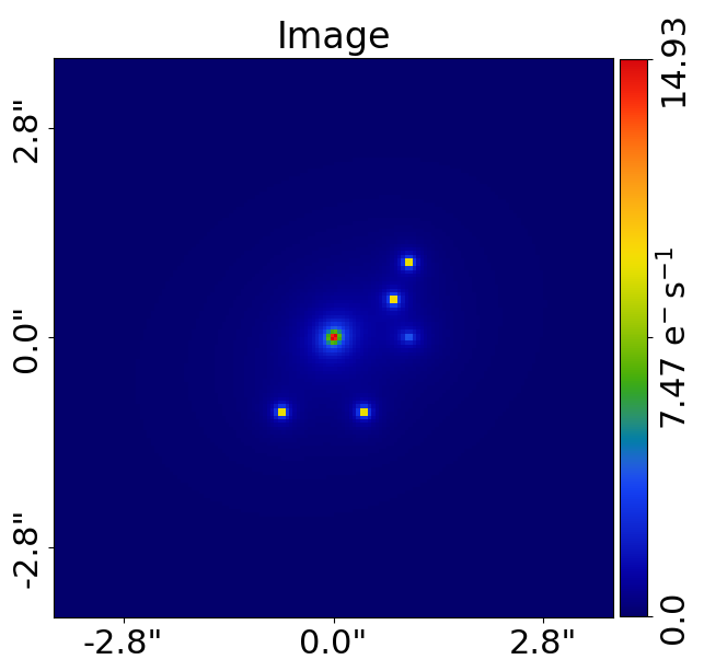
All of the objects we’ve introduced so far are highly extensible, for example a galaxy can be made up of any number of light profiles and many galaxy objects can be combined into a galaxies object.
To further illustrate this, we create a merging galaxy system with 4 star forming clumps of light, using a
SersicSph profile to make each spherical.
galaxy_0 = ag.Galaxy(
    redshift=0.5,
    bulge=ag.lp.Sersic(
        centre=(0.0, 0.0),
        ell_comps=ag.convert.ell_comps_from(axis_ratio=0.9, angle=45.0),
        intensity=0.2,
        effective_radius=0.8,
        sersic_index=4.0,
    ),
    disk=ag.lp.Exponential(
        centre=(0.0, 0.0),
        ell_comps=ag.convert.ell_comps_from(axis_ratio=0.7, angle=30.0),
        intensity=0.1,
        effective_radius=1.6,
    ),
    extra_galaxy_0=ag.lp.SersicSph(centre=(1.0, 1.0), intensity=0.5, effective_radius=0.2),
    extra_galaxy_1=ag.lp.SersicSph(centre=(0.5, 0.8), intensity=0.5, effective_radius=0.2),
    extra_galaxy_2=ag.lp.SersicSph(centre=(-1.0, -0.7), intensity=0.5, effective_radius=0.2),
    extra_galaxy_3=ag.lp.SersicSph(centre=(-1.0, 0.4), intensity=0.5, effective_radius=0.2),
)

galaxy_1 = ag.Galaxy(
    redshift=0.5,
    bulge=ag.lp.Sersic(
        centre=(0.0, 1.0),
        ell_comps=(0.0, 0.1),
        intensity=0.1,
        effective_radius=0.6,
        sersic_index=3.0,
    ),
)

galaxies = ag.Galaxies(galaxies=[galaxy_0, galaxy_1])

aplt.plot_array(array=galaxies.image_2d_from(grid=grid), title="Galaxies Image")
The image of the merging galaxy system appears as follows:
Galaxy Modeling#
Galaxy modeling is the process of fitting a physical model to imaging data in order to infer the structural and photometric properties of galaxies, such as their light distribution, size, shape, and orientation.
The primary goal of PyAutoGalaxy is to make galaxy modeling simple, scalable to large datasets, and fast, with GPU acceleration provided via JAX.
The animation below illustrates the galaxy modeling workflow. Many models are fitted to the data iteratively, progressively improving the quality of the fit until the model closely reproduces the observed image.
NOTE: Placeholder showing strong lens modeling animation used currently.
Credit: Amy Etherington
The next documentation page guides you through galaxy modeling for a variety of data types (e.g. CCD imaging at different resolutions) and scientific use-cases (e.g. galaxy morphology studies, bulge–disk decomposition).
Simulations#
Simulating galaxy images is often essential, for example to:
Practice galaxy modeling before working with real data.
Generate large training sets (e.g. for machine learning).
Test galaxy formation and structural models in a fully controlled environment.
The next documentation page guides you through how to simulate galaxies for different types of data (e.g. CCD imaging) and different modeling goals (e.g. single-component galaxies, multi-component systems).
Wrap Up#
This completes the introduction to PyAutoGalaxy, including a brief overview of the core API for galaxy light profile calculations, galaxy modeling, and data simulation.
Different users will be interested in galaxies across a range of physical scales and scientific applications (e.g. detailed structural studies, population analyses, or multi-wavelength modeling) and using different types of data (e.g. CCD imaging or interferometer observations).
The autogalaxy_workspace repository contains a wide range of examples and tutorials covering these use cases. The next documentation page helps new users identify the most appropriate starting point based on their scientific goals.