Model Cookbook#
The model cookbook provides a concise reference to model composition tools, specifically the Model
and Collection objects.
Examples using different PyAutoGalaxy API’s for model composition are provided, which produce more concise and readable code for different use-cases.
Simple Model#
A simple model we can compose has a galaxy with a linear Sersic light profile:
bulge = af.Model(ag.lp_linear.Sersic)

galaxy = af.Model(ag.Galaxy, redshift=0.5, bulge=bulge)

model = af.Collection(galaxies=af.Collection(galaxy=galaxy))
The model total_free_parameters tells us the total number of free parameters (which are fitted for via a
non-linear search), which in this case is 6. The intensity of a linear light profile is not one of them: it is
solved for by a linear inversion during every likelihood evaluation.
print(f"Model Total Free Parameters = {model.total_free_parameters}")
If we print the info attribute of the model we get information on all of the parameters and their priors.
print(model.info)
This gives the following output:
Total Free Parameters = 6

model                                                                           Collection (N=6)
    galaxies                                                                    Collection (N=6)
        galaxy                                                                  Galaxy (N=6)
            bulge                                                               Sersic (N=6)

galaxies
    galaxy
        redshift                                                                0.5
        bulge
            centre
                centre_0                                                        GaussianPrior [0], mean = 0.0, sigma = 0.3
                centre_1                                                        GaussianPrior [1], mean = 0.0, sigma = 0.3
            ell_comps
                ell_comps_0                                                     TruncatedGaussianPrior [2], mean = 0.0, sigma = 0.3, lower_limit = -1.0, upper_limit = 1.0
                ell_comps_1                                                     TruncatedGaussianPrior [3], mean = 0.0, sigma = 0.3, lower_limit = -1.0, upper_limit = 1.0
            effective_radius                                                    UniformPrior [4], lower_limit = 0.0, upper_limit = 30.0
            sersic_index                                                        UniformPrior [5], lower_limit = 0.8, upper_limit = 5.0
The same model can be drawn as a figure, which shows its structure at a glance:
af.ModelPlotter(model).figure()
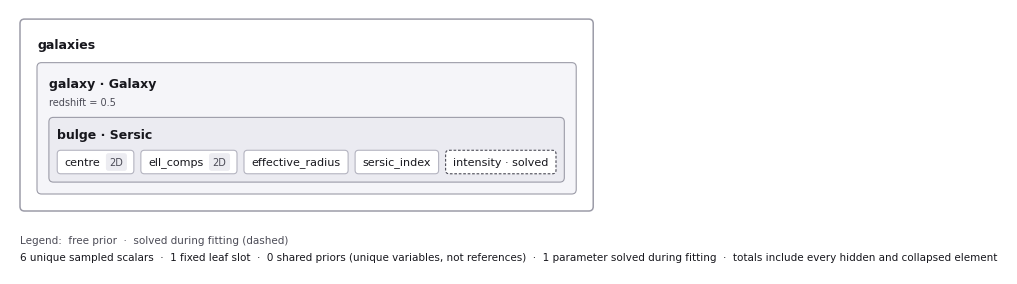
The dashed intensity · solved pill is the parameter that model.info above does not print, because it is not part
of the model: it is solved for during the fit. See Reading the figure at the end of this cookbook.
More Complex Models#
The API above can be easily extended to compose models where each galaxy has multiple light or mass profiles:
bulge = af.Model(ag.lp_linear.Sersic)
disk = af.Model(ag.lp_linear.Exponential)
bar = af.Model(ag.lp_linear.Sersic)

galaxy = af.Model(
    ag.Galaxy,
    redshift=0.5,
    bulge=bulge,
    disk=disk,
    bar=bar
)

model = af.Collection(galaxies=af.Collection(galaxy=galaxy))

af.ModelPlotter(model).figure()
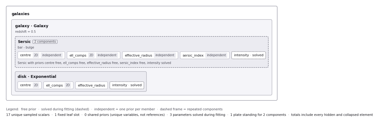
The use of the words bulge, disk and bar above are arbitrary. They can be replaced with any name you
like, e.g. bulge_0, bulge_1, star_clump, and the model will still behave in the same way.
The API can also be extended to compose models where there are multiple galaxies:
bulge = af.Model(ag.lp_linear.Sersic)

galaxy_0 = af.Model(
    ag.Galaxy,
    redshift=0.5,
    bulge=bulge,
)

bulge = af.Model(ag.lp_linear.Sersic)

galaxy_1 = af.Model(
    ag.Galaxy,
    redshift=0.5,
    bulge=bulge,
)

model = af.Collection(
    galaxies=af.Collection(
        galaxy_0=galaxy_0,
        galaxy_1=galaxy_1,
    )
)

af.ModelPlotter(model).figure()
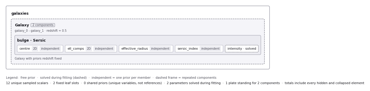
The two galaxies are identical in structure, so the figure draws them once inside a dashed plate badged
2 components rather than twice. Their parameters are badged independent: two separate priors with the same
configuration, which is not the same thing as one shared prior.
Concise API#
If a light profile is passed directly to the af.Model of a galaxy, it is automatically assigned to be a af.Model
component of the galaxy.
This means we can write the model above comprising multiple light profiles more concisely as follows:
galaxy = af.Model(
    ag.Galaxy,
    redshift=0.5,
    bulge=ag.lp_linear.Sersic,
    disk=ag.lp_linear.Exponential,
    bar=ag.lp_linear.Sersic
)

model = af.Collection(galaxies=af.Collection(galaxy=galaxy))

af.ModelPlotter(model).figure()
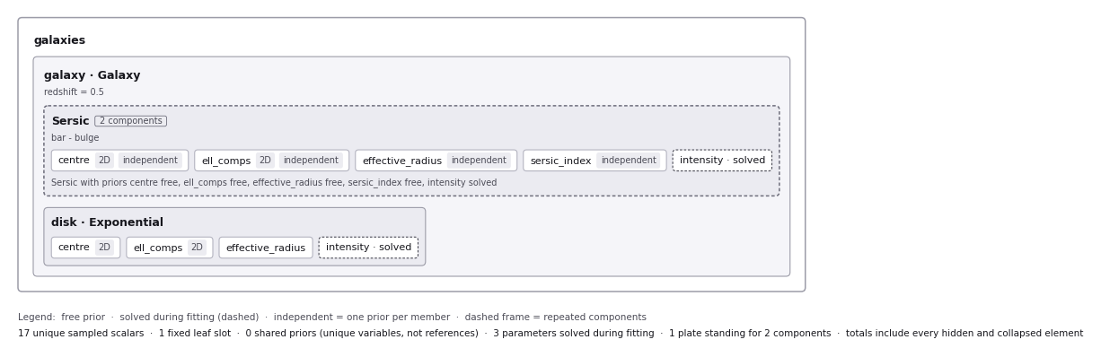
The figure is identical to the one composed the long way round, which is the point: the concise API is a shorthand for writing the model, not a different model.
Prior Customization#
We can customize the priors of the model component individual parameters as follows:
bulge = af.Model(ag.lp_linear.Sersic)
bulge.centre.centre_0 = af.UniformPrior(lower_limit=-0.1, upper_limit=0.1)
bulge.centre.centre_1 = af.UniformPrior(lower_limit=-0.1, upper_limit=0.1)
bulge.sersic_index = af.TruncatedGaussianPrior(
    mean=4.0, sigma=1.0, lower_limit=1.0, upper_limit=8.0
)

galaxy = af.Model(
    ag.Galaxy,
    redshift=0.5,
    bulge=bulge,
)

model = af.Collection(galaxies=af.Collection(galaxy=galaxy))

af.ModelPlotter(model).figure()
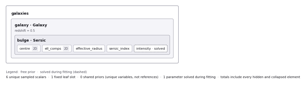
Customizing a prior does not change a parameter’s state: every parameter above is still sampled, so the figure is
unchanged by the customization. Print model.info, or call af.ModelPlotter(model).figure(detail="priors"), to see
the prior on each parameter.
Model Customization#
We can customize the model parameters in a number of different ways, as shown below:
bulge = af.Model(ag.lp_linear.Sersic)
disk = af.Model(ag.lp_linear.Exponential)

# Parameter Pairing: Pair the centre of the bulge and disk together, reducing
# the complexity of non-linear parameter space by N = 2

bulge.centre = disk.centre

# Parameter Fixing: Fix the sersic_index of the bulge to a value of 4, reducing
# the complexity of non-linear parameter space by N = 1

bulge.sersic_index = 4.0

# Parameter Offsets: Make the bulge effective_radius the same value as
# the disk but with an offset.

bulge.effective_radius = disk.effective_radius + 0.1

galaxy = af.Model(
    ag.Galaxy,
    redshift=0.5,
    bulge=bulge,
    disk=disk,
)

model = af.Collection(galaxies=af.Collection(galaxy=galaxy))

# Assert that the effective radius of the bulge is larger than that of the disk.
# (Assertions can only be added at the end of model composition, after all components
# have been brought together in a `Collection`.
model.add_assertion(model.galaxies.galaxy.bulge.effective_radius > model.galaxies.galaxy.disk.effective_radius)

# Assert that the bulge effective radius is below 3.0":
model.add_assertion(model.galaxies.galaxy.bulge.effective_radius < 3.0)

af.ModelPlotter(model).figure()
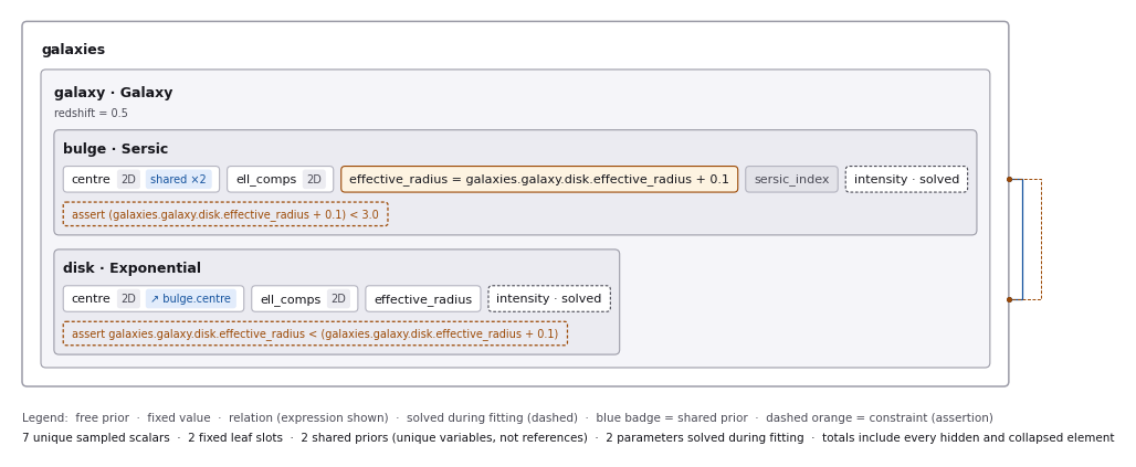
This is the stage where the figure earns its keep: the paired centre is drawn once on its owner with a badge and a
link from the component that reuses it, the fixed sersic_index is a grey pill, the offset effective_radius carries
its defining expression, and each assertion is a compact label naming both of its operands.
Reading the figure#
The figure is the map; model.info is the legend. The map shows the shape of the model — which components
contain which, which parameters are shared, fixed, related or solved — and the legend gives the numbers: the prior on
every parameter, and the exact value of every fixed one.
The contract between them is explicit: every displayed model element resolves to its corresponding path or grouped
paths in model.info, and every omission and every added annotation (solved, missing) is called out on the figure
itself. It is deliberately not a line-for-line correspondence — the figure partitions by component, while
model.info groups per parameter, so one plate of thirty components can correspond to a single 0 - 29 block in the
text.
A solved pill has no counterpart in model.info at all: it is additional information. The intensity of a linear
light profile (ag.lp_linear.*, and every member of an ag.lp_basis.Basis built from them) is solved for by the
inversion at every likelihood evaluation, so it has no prior and is absent from the text. A Basis declares no solved
amplitude of its own — the solved intensities belong to its member profiles, one per member.
The background tints follow nesting depth only. They are decorative: they help you see which card sits inside which, and they carry no information about the class family of a component. A light profile and a mass profile at the same depth are tinted identically.
Available Model Components#
The light profiles, mass profiles and other components that can be used for galaxy modeling are given at the following API documentation pages:
JSon Outputs#
After a model is composed, it can easily be output to a .json file on hard-disk in a readable structure:
import os
import json

model_path = path.join("path", "to", "model", "json")

os.makedirs(model_path, exist_ok=True)

model_file = path.join(model_path, "model.json")

with open(model_file, "w+") as f:
    json.dump(model.dict(), f, indent=4)
We can load the model from its .json file.
model = af.Model.from_json(file=model_file)
This means in PyAutoGalaxy one can write a model in a script, save it to hard disk and load it elsewhere, as well as manually customize it in the .json file directory.
Many Profile Models (Advanced)#
Features such as the Multi Gaussian Expansion (MGE) and shapelets compose models consisting of 50 - 500+ light profiles.
The following example notebooks show how to compose and fit these models:
https://github.com/PyAutoLabs/autogalaxy_workspace/blob/main/notebooks/imaging/features/multi_gaussian_expansion/modeling.ipynb https://github.com/PyAutoLabs/autogalaxy_workspace/blob/main/notebooks/imaging/features/shapelets/modeling.ipynb
Model Linking (Advanced)#
When performing non-linear search chaining, the inferred model of one phase can be linked to the model.
The following example notebooks show how to compose and fit these models:
Across Datasets (Advanced)#
When fitting multiple datasets, model can be composed where the same model component are used across the datasets but certain parameters are free to vary across the datasets.
The following example notebooks show how to compose and fit these models:
Relations (Advanced)#
We can compose models where the free parameter(s) vary according to a user-specified function (e.g. y = mx +c -> intensity = (m * wavelength) + c across the datasets.
The following example notebooks show how to compose and fit these models:
PyAutoFit API#
PyAutoFit is a general model composition library which offers even more ways to compose models not detailed in this cookbook.
The PyAutoFit model composition cookbooks detail this API in more detail:
https://pyautofit.readthedocs.io/en/latest/cookbooks/model.html https://pyautofit.readthedocs.io/en/latest/cookbooks/multi_level_model.html
Wrap Up#
This cookbook shows how to compose simple models using the af.Model() and af.Collection() objects.