Fitting Data

PyAutoGalaxy uses Plane objects to represent multi-galaxy systems.

We now use these objects to fit Imaging data of a galaxy.

Loading Data

We we begin by loading a galaxy dataset from .fits files, which is the dataset we will use to demonstrate fitting.

dataset_name = "light_sersic"
dataset_path = path.join("dataset", "imaging", dataset_name)

dataset = ag.Imaging.from_fits(
    data_path=path.join(dataset_path, "data.fits"),
    psf_path=path.join(dataset_path, "psf.fits"),
    noise_map_path=path.join(dataset_path, "noise_map.fits"),
    pixel_scales=0.1,
)

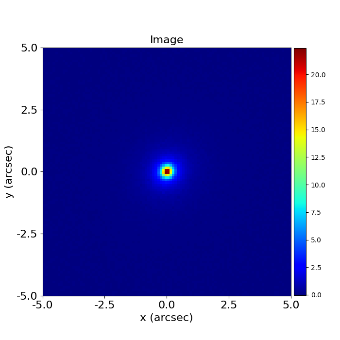
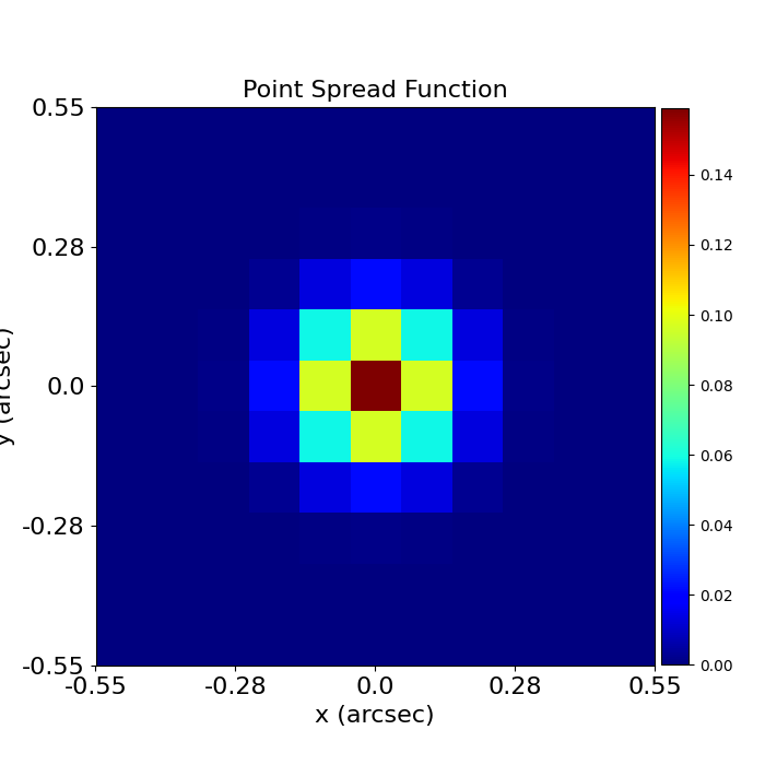
dataset_plotter = aplt.ImagingPlotter(dataset=dataset)
dataset_plotter.figures_2d(data=True, noise_map=True, psf=True)

Here’s what our image, noise_map and psf (point-spread function) look like:

Masking

We next mask the data, so that regions where there is no signal (e.g. the edges) are omitted from the fit.

To do this we can use a Mask2D object, which for this example we’ll create as a 3.0” circle.

mask = ag.Mask2D.circular(
    shape_native=dataset.shape_native, pixel_scales=dataset.pixel_scales, radius=3.0
)

dataset = dataset.apply_mask(mask=mask)

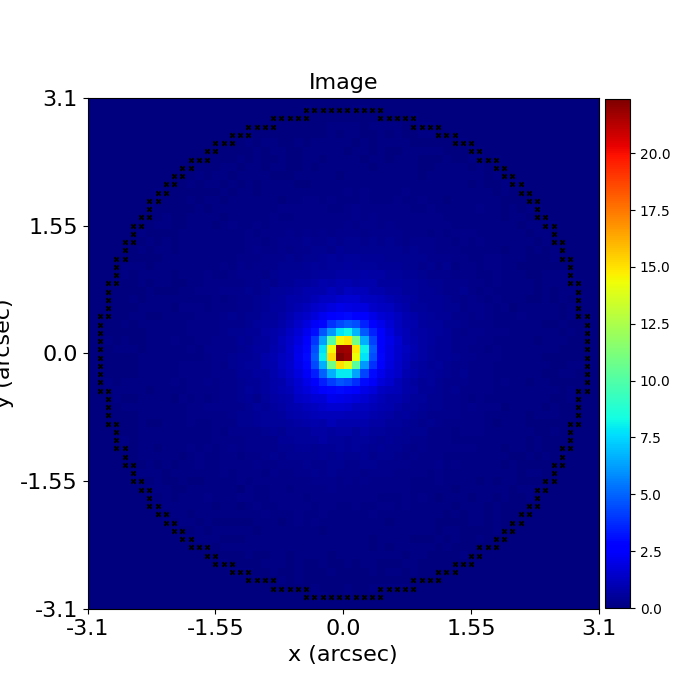
dataset_plotter = aplt.ImagingPlotter(dataset=dataset)
dataset_plotter.figures_2d(data=True)

Here is what our image looks like with the mask applied, where PyAutoGalaxy has automatically zoomed around the Mask2D to make the lensed source appear bigger:

Fitting

Following the previous overview, we can make a plane from a collection of LightProfile and Galaxy objects.

The combination of LightProfile’s below is the same as those used to generate the simulated dataset we loaded above.

It therefore produces a plane whose image looks exactly like the dataset.

galaxy = ag.Galaxy(
    redshift=0.5,
    bulge=ag.lp.Sersic(
        centre=(0.0, 0.0),
        ell_comps=ag.convert.ell_comps_from(axis_ratio=0.9, angle=45.0),
        intensity=1.0,
        effective_radius=0.8,
        sersic_index=4.0,
    ),
)

plane = ag.Plane(galaxies=[galaxy])

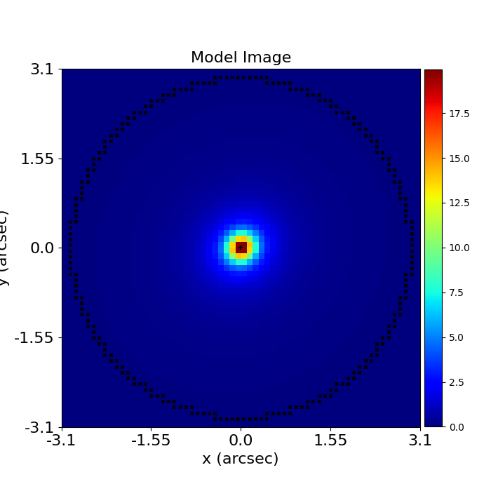
We now use the FitImaging object to fit this plane to the dataset.

The fit performs the necessary tasks to create the model_image we fit the data with, such as blurring the plane`s image with the Imaging Point Spread Function (PSF). We can see this by comparing the plane`s image (which isn’t PSF convolved) and the fit`s model image (which is).

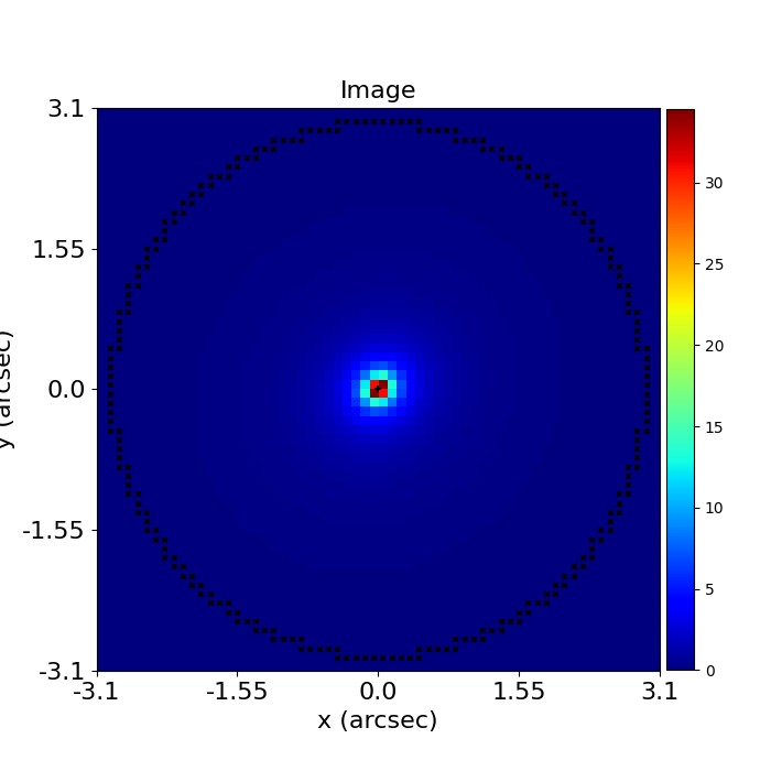
fit = ag.FitImaging(dataset=dataset, plane=plane)

fit_plotter = aplt.FitImagingPlotter(fit=fit)
fit_plotter.figures_2d(model_image=True)

Here is how the Plane’s image of the galaxy and the FitImaging’s model-image look.

Note how the model-image has been blurred with the PSF of our dataset:

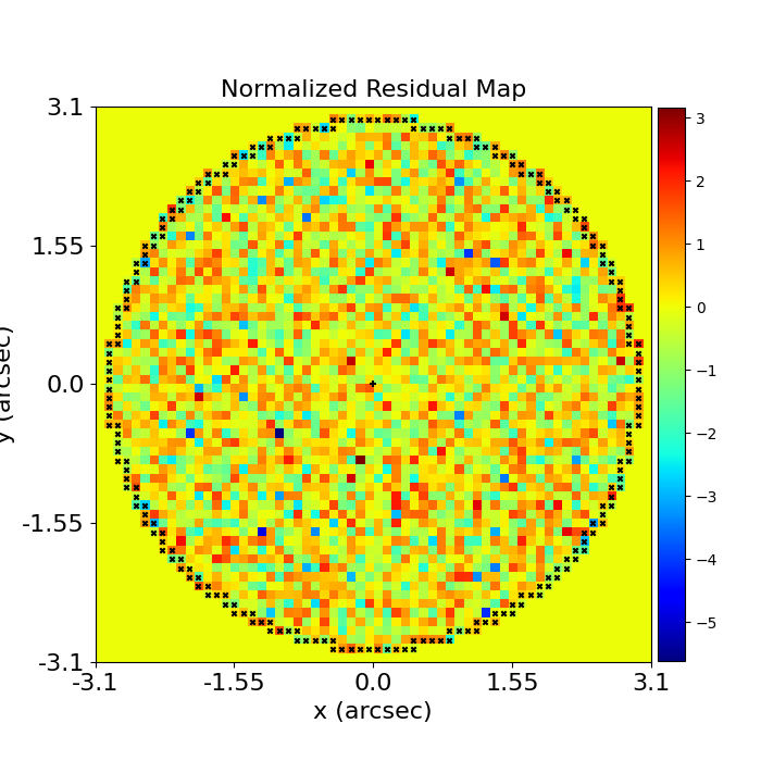
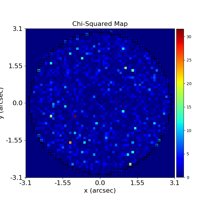
The fit creates the following:

• The residual_map: The model_image subtracted from the observed dataset`s image.

• The normalized_residual_map: The residual_map `divided by the observed dataset’s `noise_map.

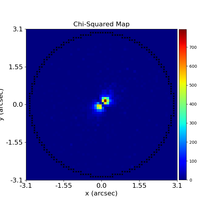
• The chi_squared_map: The normalized_residual_map squared.

We can plot all three of these quantities

fit_plotter = aplt.FitImagingPlotter(fit=fit)

fit_plotter.figures_2d(
    residual_map=True,
    normalized_residual_map=True,
    chi_squared_map=True
)

For a good model where the model image and plane are representative of the galaxy system the residuals, normalized residuals and chi-squared are minimized:

The overall quality of the fit is quantified with the log_likelihood:

print(fit.log_likelihood)

Bad Fit

In contrast, a bad lens model will show features in the residual-map and chi-squareds:

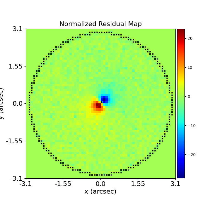
If we can find a Plane that produces a high log likelihood, we’ll have a model which is representative of our galaxy data!

This task, called modeling, is covered in the next API overview.

Wrap Up

A more detailed description of PyAutoGalaxy’s fitting methods (including a description of terms like ‘residuals’, ‘chi-sqaured’ and ‘likelihood’) are given in chapter 1 of the HowToGalaxy tutorials, which I strongly advise new users check out!

Checkout the

tutorials section of the readthedocs!