Modeling#
We can use a Plane to fit data of a galaxy and quantify its goodness-of-fit via a
log_likelihood.
Of course, when observe an image of a galaxy, we have no idea what combination of
LightProfile’s will produce a model-image that looks like the galaxy we observed:
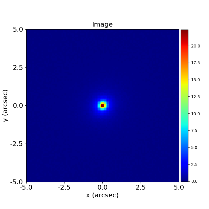
The task of finding these LightProfiles’is called modeling.
PyAutoFit#
Modeling uses the probabilistic programming language PyAutoFit, an open-source Python framework that allows complex model fitting techniques to be straightforwardly integrated into scientific modeling software. Check it out if you are interested in developing your own software to perform advanced model-fitting!
We import it separately to PyAutoGalaxy
import autofit as af
Model Composition#
We compose the model that we fit to the data using a Model object, which behaves analogously to the Galaxy,
and LightProfile used previously, however their parameters are not specified and are instead
determined by a fitting procedure.
galaxy = af.Model(
    ag.Galaxy, redshift=0.5, bulge=ag.lp.Sersic, disk=ag.lp.Exponential
)
We put the model galaxy above into a Collection, which is the model we will fit. Note how we could easily extend this object to compose complex models containing many galaxies.
The reason we create separate Collection’s for the galaxies and model is so that the model can be extended to include other components than just galaxies.
galaxies = af.Collection(galaxy=galaxy)
model = af.Collection(galaxies=galaxies)
In this example we therefore fit a model where:
The galaxy’s bulge is a parametric Sersic bulge [7 parameters].
The galaxy’s disk is a parametric Exponential disk [6 parameters].
The redshifts of the galaxy (z=0.5) is fixed.
Printing the info attribute of the model shows us this is the model we are fitting, and shows us the free
parameters and their priors:
print(model.info)
This gives the following output:
galaxies
    galaxy
        redshift                                   0.5
        bulge
            centre
                centre_0                           GaussianPrior, mean = 0.0, sigma = 0.3
                centre_1                           GaussianPrior, mean = 0.0, sigma = 0.3
            ell_comps
                ell_comps_0                        GaussianPrior, mean = 0.0, sigma = 0.5
                ell_comps_1                        GaussianPrior, mean = 0.0, sigma = 0.5
            intensity                              LogUniformPrior, lower_limit = 1e-06, upper_limit = 1000000.0
            effective_radius                       UniformPrior, lower_limit = 0.0, upper_limit = 30.0
            sersic_index                           UniformPrior, lower_limit = 0.8, upper_limit = 5.0
        disk
            centre
                centre_0                           GaussianPrior, mean = 0.0, sigma = 0.3
                centre_1                           GaussianPrior, mean = 0.0, sigma = 0.3
            ell_comps
                ell_comps_0                        GaussianPrior, mean = 0.0, sigma = 0.5
                ell_comps_1                        GaussianPrior, mean = 0.0, sigma = 0.5
            intensity                              LogUniformPrior, lower_limit = 1e-06, upper_limit = 1000000.0
            effective_radius                       UniformPrior, lower_limit = 0.0, upper_limit = 30.0
Non-linear Search#
We now choose the non-linear search, which is the fitting method used to determine the set of LightProfile (e.g. bulge and disk) parameters that best-fit our data.
In this example we use dynesty (https://github.com/joshspeagle/dynesty), a nested sampling algorithm that is very effective at modeling.
search = af.Nautilus(name="search_example")
PyAutoGalaxy supports many model-fitting algorithms, including maximum likelihood estimators and MCMC, which are documented throughout the workspace.
Analysis#
We next create an AnalysisImaging object, which contains the log likelihood function that the non-linear
search calls to fit the model to the data.
analysis = ag.AnalysisImaging(dataset=dataset)
Run Times#
modeling can be a computationally expensive process. When fitting complex models to high resolution datasets run times can be of order hours, days, weeks or even months.
Run times are dictated by two factors:
The log likelihood evaluation time: the time it takes for a single
instanceof the model to be fitted to the dataset such that a log likelihood is returned.The number of iterations (e.g. log likelihood evaluations) performed by the non-linear search: more complex lens models require more iterations to converge to a solution.
The log likelihood evaluation time can be estimated before a fit using the profile_log_likelihood_function method,
which returns two dictionaries containing the run-times and information about the fit.
run_time_dict, info_dict = analysis.profile_log_likelihood_function(
    instance=model.random_instance()
)
The overall log likelihood evaluation time is given by the fit_time key.
For this example, it is ~0.01 seconds, which is extremely fast for modeling. More advanced lens modeling features (e.g. shapelets, multi Gaussian expansions, pixelizations) have slower log likelihood evaluation times (1-3 seconds), and you should be wary of this when using these features.
The run_time_dict has a break-down of the run-time of every individual function call in the log likelihood
function, whereas the info_dict stores information about the data which drives the run-time (e.g. number of
image-pixels in the mask, the shape of the PSF, etc.).
print(f"Log Likelihood Evaluation Time (second) = {run_time_dict['fit_time']}")
This gives an output of ~0.01 seconds.
To estimate the expected overall run time of the model-fit we multiply the log likelihood evaluation time by an estimate of the number of iterations the non-linear search will perform.
Estimating this quantity is more tricky, as it varies depending on the model complexity (e.g. number of parameters) and the properties of the dataset and model being fitted.
For this example, we conservatively estimate that the non-linear search will perform ~10000 iterations per free parameter in the model. This is an upper limit, with models typically converge in far fewer iterations.
If you perform the fit over multiple CPUs, you can divide the run time by the number of cores to get an estimate of
the time it will take to fit the model. Parallelization with Nautilus scales well, it speeds up the model-fit by the
number_of_cores for N < 8 CPUs and roughly 0.5*number_of_cores for N > 8 CPUs. This scaling continues
for N> 50 CPUs, meaning that with super computing facilities you can always achieve fast run times!
print(
    "Estimated Run Time Upper Limit (seconds) = ",
    (run_time_dict["fit_time"] * model.total_free_parameters * 10000)
    / search.number_of_cores,
)
Model-Fit#
To perform the model-fit we pass the model and analysis to the search’s fit method. This will output results (e.g., dynesty samples, model parameters, visualization) to hard-disk.
result = search.fit(model=model, analysis=analysis)
The non-linear search fits the model by guessing many models over and over iteratively, using the models which give a good fit to the data to guide it where to guess subsequent model.
An animation of a non-linear search is shown below, although this is for a strong gravitational using PyAutoGalaxy’s child project PyAutoLens. Updating the animation for a galaxy is on the PyAutoGalaxy to-do list!
We can see that initial models give a poor fit to the data but gradually improve (increasing the likelihood) as more iterations are performed.
Credit: Amy Etherington
Results#
Once a model-fit is running, PyAutoGalaxy outputs the results of the search to hard-disk on-the-fly. This includes model parameter estimates with errors non-linear samples and the visualization of the best-fit model inferred by the search so far.
The fit above returns a Result object, which includes lots of information on the model.
The info attribute can be printed to give the results in a readable format:
print(result_list.info)
This gives the following output:
Bayesian Evidence                              4910.81446407
Maximum Log Likelihood                         5010.64422962
Maximum Log Posterior                          975179.18825227

model                                          Collection (N=13)
    galaxies                                   Collection (N=13)
        galaxy                                 Galaxy (N=13)
            bulge                              Sersic (N=7)
            disk                               Exponential (N=6)

Maximum Log Likelihood Model:

galaxies
    galaxy
        bulge
            centre
                centre_0                       -0.002
                centre_1                       0.001
            ell_comps
                ell_comps_0             0.056
                ell_comps_1             -0.009
            intensity                          0.757
            effective_radius                   0.708
            sersic_index                       3.554
        disk
            centre
                centre_0                       0.001
                centre_1                       -0.004
            ell_comps
                ell_comps_0             0.155
                ell_comps_1             0.091
            intensity                          0.500
            effective_radius                   1.554


Summary (3.0 sigma limits):

galaxies
    galaxy
        bulge
            centre
                centre_0                       -0.0028 (-0.0051, 0.0005)
                centre_1                       0.0014 (-0.0013, 0.0038)
            ell_comps
                ell_comps_0             0.0542 (0.0411, 0.0641)
                ell_comps_1             -0.0066 (-0.0189, 0.0078)
            intensity                          0.5153 (0.3576, 0.7726)
            effective_radius                   0.8984 (0.7042, 1.1218)
            sersic_index                       4.0917 (3.5170, 4.6985)
        disk
            centre
                centre_0                       0.0020 (-0.0062, 0.0095)
                centre_1                       -0.0038 (-0.0122, 0.0061)
            ell_comps
                ell_comps_0             0.1608 (0.1539, 0.1710)
                ell_comps_1             0.0942 (0.0874, 0.1027)
            intensity                          0.4912 (0.4657, 0.5121)
            effective_radius                   1.5250 (1.4828, 1.5636)


Summary (1.0 sigma limits):

galaxies
    galaxy
        bulge
            centre
                centre_0                       -0.0028 (-0.0036, -0.0020)
                centre_1                       0.0014 (0.0005, 0.0024)
            ell_comps
                ell_comps_0             0.0542 (0.0503, 0.0577)
                ell_comps_1             -0.0066 (-0.0103, -0.0029)
            intensity                          0.5153 (0.4382, 0.6041)
            effective_radius                   0.8984 (0.8109, 0.9900)
            sersic_index                       4.0917 (3.8877, 4.3431)
        disk
            centre
                centre_0                       0.0020 (-0.0004, 0.0046)
                centre_1                       -0.0038 (-0.0068, -0.0009)
            ell_comps
                ell_comps_0             0.1608 (0.1575, 0.1638)
                ell_comps_1             0.0942 (0.0916, 0.0967)
            intensity                          0.4912 (0.4827, 0.4986)
            effective_radius                   1.5250 (1.5058, 1.5399)

instances

galaxies
    galaxy
        redshift                               0.5
This result contains the full posterior information of our non-linear search, including all parameter samples, log likelihood values and tools to compute the errors on the model.
This is contained in the Samples object. Below, we show how to print the median PDF parameter estimates, but
many different results are available and illustrated in the results package of the workspace.
samples = result.samples

median_pdf_instance = samples.median_pdf()

print("Median PDF Model Instances: \n")
print(median_pdf_instance, "\n")
print(median_pdf_instance.galaxies.galaxy.bulge)
print()
PyAutoGalaxy includes many visualization tools for plotting the results of a non-linear search, for example we can make a corner plot of the probability density function (PDF):
search_plotter = aplt.DynestyPlotter(samples=result.samples)
search_plotter.cornerplot()
Here is an example of how a PDF estimated for a model appears:

The result also contains the maximum log likelihood Plane and FitImaging objects and which can easily be
plotted.
plane_plotter = aplt.PlanePlotter(plane=result.max_log_likelihood_plane, grid=mask.derive_grid.masked)
plane_plotter.subplot_plane()
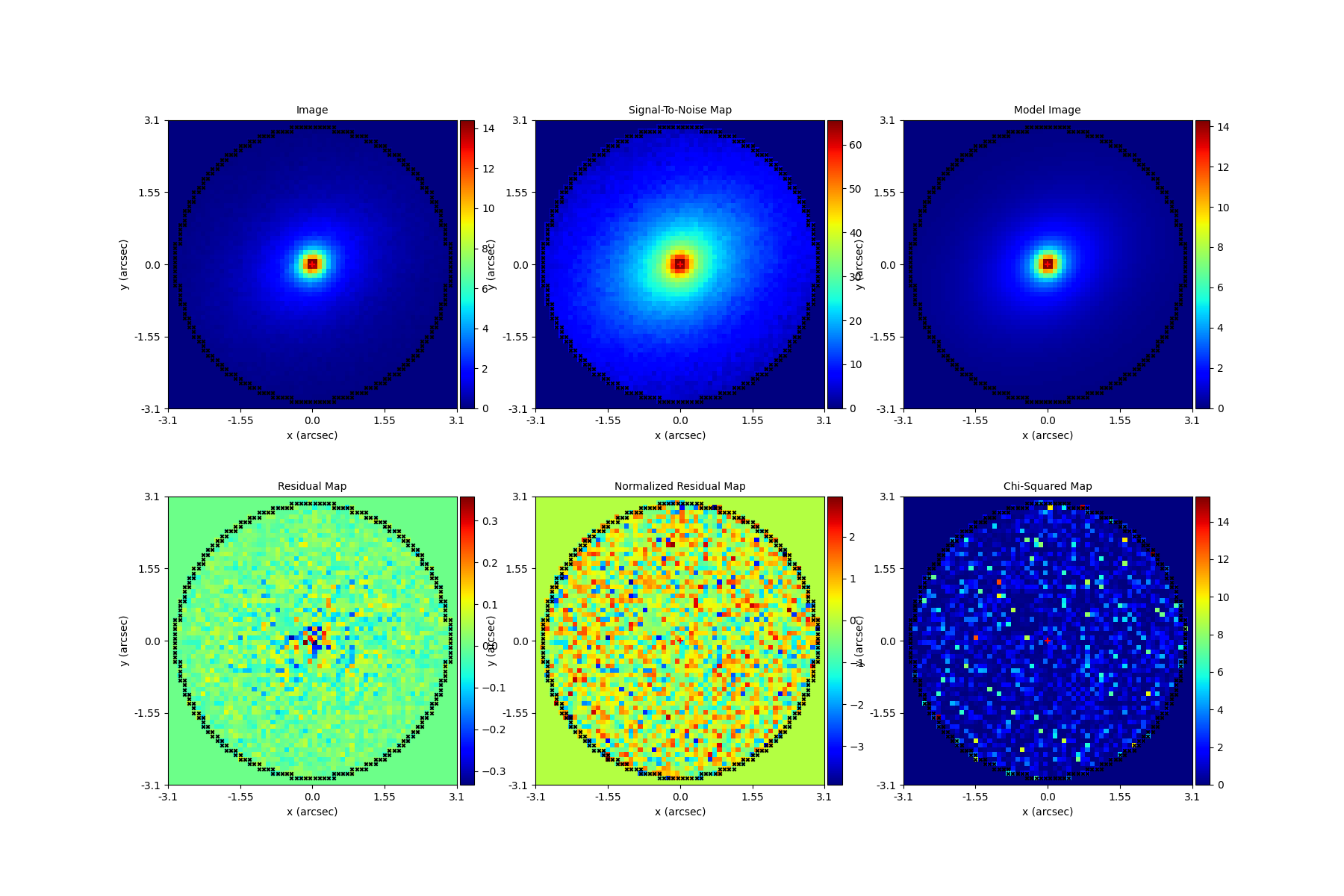
fit_plotter = aplt.FitImagingPlotter(fit=result.max_log_likelihood_fit)
fit_plotter.subplot_fit()
Here’s what the model-fit of the model which maximizes the log likelihood looks like, providing good residuals and low chi-squared values:
The package autogalaxy_workspace/*/results contains a full description of all information contained
in a Result.
Model Customization#
The Model can be fully customized, making it simple to parameterize and fit many different models
using any combination of light profiles:
galaxy_model = af.Model(
    ag.Galaxy,
    redshift=0.5,
    bulge=ag.lp.DevVaucouleurs,
    disk = ag.lp.Sersic,
    bar=ag.lp.Gaussian,
    clump_0=ag.lp.ElsonFreeFall,
    clump_1=ag.lp.ElsonFreeFall,
)

"""
This aligns the bulge and disk centres in the galaxy model, reducing the
number of free parameter fitted for by Dynesty by 2.
"""
galaxy_model.bulge.centre = galaxy_model.disk.centre

"""
This fixes the galaxy bulge light profile's effective radius to a value of
0.8 arc-seconds, removing another free parameter.
"""
galaxy_model.bulge.effective_radius = 0.8

"""
This forces the light profile disk's effective radius to be above 3.0.
"""
galaxy_model.bulge.add_assertion(galaxy_model.disk.effective_radius > 3.0)
Linear Light Profiles#
PyAutoGalaxy supports ‘linear light profiles’, where the intensity parameters of all parametric components are
solved via linear algebra every time the model is fitted using a process called an inversion. This inversion always
computes intensity values that give the best fit to the data (e.g. they maximize the likelihood) given the other
parameter values of the light profile.
The intensity parameter of each light profile is therefore not a free parameter in the model-fit, reducing the
dimensionality of non-linear parameter space by the number of light profiles (in the example below by 3) and removing
the degeneracies that occur between the intnensity and other light profile
parameters (e.g. effective_radius, sersic_index).
For complex models, linear light profiles are a powerful way to simplify the parameter space to ensure the best-fit model is inferred.
sersic_linear = ag.lp_linear.Sersic()

galaxy_model_linear = af.Model(
    ag.Galaxy,
    redshift=0.5,
    bulge=ag.lp_linear.DevVaucouleurs,
    disk=ag.lp_linear.Sersic,
    bar=ag.lp_linear.Gaussian,
)
Basis Functions#
A natural extension of linear light profiles are basis functions, which group many linear light profiles together in order to capture complex and irregular structures in a galaxy’s emission.
Using a clever model parameterization a basis can be composed which corresponds to just N = 3-6 non-linar parameters, making model-fitting efficient and robust.
Below, we compose a basis of 10 Gaussians which all share the same centre and ell_comps. Their sigma values are set via the relation y = a + (log10(i+1) + b), where i is the Gaussian index and a and b are free parameters.
Because a and b are free parameters (as opposed to sigma which can assume many values), we are able to compose and fit Basis objects which can capture very complex light distributions with just N = 5-10 non-linear parameters!
bulge_a = af.UniformPrior(lower_limit=0.0, upper_limit=0.2)
bulge_b = af.UniformPrior(lower_limit=0.0, upper_limit=10.0)

gaussians_bulge = af.Collection(af.Model(ag.lp_linear.Gaussian) for _ in range(10))

for i, gaussian in enumerate(gaussians_bulge):

    gaussian.centre = gaussians_bulge[0].centre
    gaussian.ell_comps = gaussians_bulge[0].ell_comps
    gaussian.sigma = bulge_a + (bulge_b * np.log10(i+1))

bulge = af.Model(
    ag.lp_basis.Basis, light_profile_list=gaussians_bulge,
)
The bulge’s info attribute describes the basis model composition:
print(bulge.info)
Below is a snippet of the model, showing that different Gaussians are in the model parameterization:
Total Free Parameters = 6

model                                                                           Basis (N=6)
    light_profile_list                                                          Collection (N=6)
        0                                                                       Gaussian (N=6)
            sigma                                                               SumPrior (N=2)
                other                                                           MultiplePrior (N=1)
        1                                                                       Gaussian (N=6)
            sigma                                                               SumPrior (N=2)
                other                                                           MultiplePrior (N=1)
        2                                                                       Gaussian (N=6)
        ...
        trimmed for conciseness
        ...


light_profile_list
    0
        centre
            centre_0                                                            GaussianPrior, mean = 0.0, sigma = 0.3
            centre_1                                                            GaussianPrior, mean = 0.0, sigma = 0.3
        ell_comps
            ell_comps_0                                                  GaussianPrior, mean = 0.0, sigma = 0.3
            ell_comps_1                                                  GaussianPrior, mean = 0.0, sigma = 0.3
        sigma
            bulge_a                                                             UniformPrior, lower_limit = 0.0, upper_limit = 0.2
            other
                bulge_b                                                         UniformPrior, lower_limit = 0.0, upper_limit = 10.0
                other                                                           0.0
    1
        centre
            centre_0                                                            GaussianPrior, mean = 0.0, sigma = 0.3
            centre_1                                                            GaussianPrior, mean = 0.0, sigma = 0.3
        ell_comps
            ell_comps_0                                                  GaussianPrior, mean = 0.0, sigma = 0.3
            ell_comps_1                                                  GaussianPrior, mean = 0.0, sigma = 0.3
        sigma
            bulge_a                                                             UniformPrior, lower_limit = 0.0, upper_limit = 0.2
            other
                bulge_b                                                         UniformPrior, lower_limit = 0.0, upper_limit = 10.0
                other                                                           0.3010299956639812
    2
    ...
    trimmed for conciseness
    ...
PyAutoGalaxy also supports Shapelet basis functions, which are appropriate for capturing exponential / disk-like features in a galaxy.
This is illustrated in full on the autogalaxy_workspace in the example
script autogalaxy_workspace/scripts/imaging/modeling/advanced/shapelets.py .
PyAutoGalaxy can also apply Bayesian regularization to Basis functions, which smooths the linear light profiles (e.g. the Gaussians) in order to prevent over-fitting noise.
bulge = af.Model(
    al.lp_basis.Basis, light_profile_list=gaussians_lens, regularization=al.reg.Constant
)
Wrap-Up#
Chapters 2 and 3 HowToGalaxy lecture series give a comprehensive description of modeling, including a description of what a non-linear search is and strategies to fit complex model to data in efficient and robust ways.