Galaxies#
Nearly a century ago, Edwin Hubble famously classified galaxies into three distinct groups: ellipticals, spirals and irregulars. Today, by analysing millions of galaxies with advanced image processing techniques Astronomers have expanded on this picture and revealed the rich diversity of galaxy morphology both in the nearby and distant Universe.
PyAutoGalaxy is an open-source Python package for the multi-wavelength analysis of the morphologies of large
galaxy samples.
To use PyAutoGalaxy we first import autogalaxy and the plot module.
import autogalaxy as al
import autogalaxy.plot as aplt
Grids#
To describe the luminous emission of galaxies, PyAutoGalaxy uses Grid2D data structures, which are two-dimensional Cartesian grids of (y,x) coordinates.
Below, we make and plot a uniform Cartesian grid (the pixel_scales describes the conversion from pixel
units to arc-seconds):
grid = ag.Grid2D.uniform(
    shape_native=(100, 100),
    pixel_scales=0.1,
)

grid_plotter = aplt.Grid2DPlotter(grid=grid)
grid_plotter.figure_2d()
import autogalaxy as ag


grid = ag.Grid2D.uniform(
    shape_native=(100, 100),
    pixel_scales=0.1,
)

grid_plotter = aplt.Grid2DPlotter(grid=grid)
grid_plotter.figure_2d()
This is what our Grid2D looks like:

Light Profiles#
We will use this Grid2D’s coordinates to evaluate the galaxy’s morphology. We therefore need analytic functions representing a galaxy’s light distribution(s).
For this, PyAutoGalaxy uses LightProfile objects, for example the Sersic LightProfile object which represents a light distribution:
sersic_light_profile = al.lp.Sersic(
    centre=(0.0, 0.0),
    ell_comps=(0.1, 0.1),
    intensity=0.05,
    effective_radius=2.0,
    sersic_index=4.0,
)
By passing this profile a Grid2D, we evaluate the light at every (y,x) coordinate on the Grid2D and create an image of the LightProfile.
image = sersic_light_profile.image_2d_from(grid=grid)
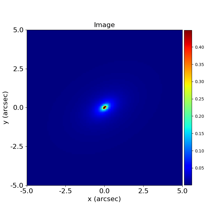
The PyAutoGalaxy plot module provides methods for plotting objects and their properties, like the LightProfile’s image.
light_profile_plotter = aplt.LightProfilePlotter(
    light_profile=sersic_light_profile, grid=grid
)
light_profile_plotter.figures_2d(image=True)
The light profile’s image appears as shown below:
Galaxies#
A Galaxy object is a collection of LightProfile objects at a given redshift.
The code below creates a galaxy which is made of two components, a bulge and disk.
bulge = ag.lp.Sersic(
    centre=(0.0, 0.0),
    ell_comps=ag.convert.ell_comps_from(axis_ratio=0.9, angle=45.0),
    intensity=1.0,
    effective_radius=0.6,
    sersic_index=3.0,
)

disk = ag.lp.Exponential(
    centre=(0.0, 0.0),
    ell_comps=ag.convert.ell_comps_from(axis_ratio=0.7, angle=30.0),
    intensity=0.5,
    effective_radius=1.6,
)

galaxy = ag.Galaxy(redshift=0.5, bulge=bulge, disk=disk)
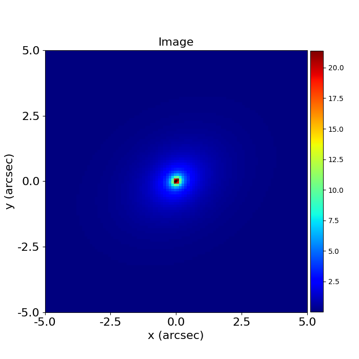
We can create an image the galaxy by passing it the 2D grid above.
image = galaxy.image_2d_from(grid=grid)
The PyAutoGalaxy plot module provides methods for plotting galaxies.
Below, we plot its image, which is the sum of the bulge and disk components.
galaxy_plotter = aplt.GalaxyPlotter(galaxy=galaxy, grid=grid)
galaxy_plotter.figures_2d(image=True)
The galaxy, with both a bulge and disk, appears as follows
Plane#
If our observation contains multiple galaxies, we create a Plane object to represent all galaxies.
By passing Galaxy objects to a Plane, PyAutoGalaxy groups them to indicate they are at the same redshift.
galaxy_0 = ag.Galaxy(
    redshift=0.5,
    bulge=ag.lp.Sersic(
        centre=(0.0, -1.0),
        ell_comps=(0.25, 0.1),
        intensity=0.1,
        effective_radius=0.8,
        sersic_index=2.5,
    ),
)

galaxy_1 = ag.Galaxy(
    redshift=0.5,
    bulge=ag.lp.Sersic(
        centre=(0.0, 1.0),
        ell_comps=(0.0, 0.1),
        intensity=0.1,
        effective_radius=0.6,
        sersic_index=3.0,
    ),
)

plane = ag.Plane(galaxies=[galaxy_0, galaxy_1])
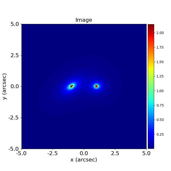
The image of the plane consists of all galaxies.
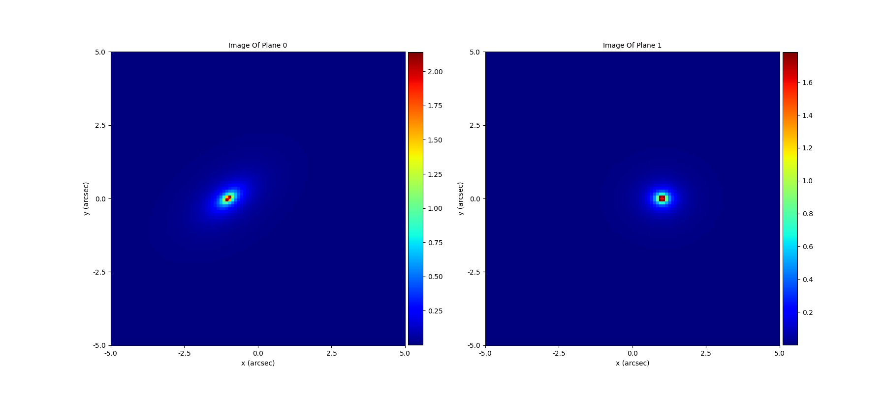
PyAutoGalaxy plot tools allow us to plot this image or a subplot containing images of each individual galaxy.
image = plane.image_2d_from(grid=grid)

plane_plotter = aplt.PlanePlotter(plane=plane, grid=grid)
plane_plotter.figures_2d(image=True)
plane_plotter.subplot_galaxy_images()
The plane image shows both galaxies:
Whereas the subplot has panels for each individual galaxy:
The galaxy, with both a bulge and disk, appears as follows
Extending Objects#
The PyAutoGalaxy API isn designed such that all of the objects introduced above are extensible. Galaxy objects can take many LightProfile’s and Plane’s many Galaxy’s.
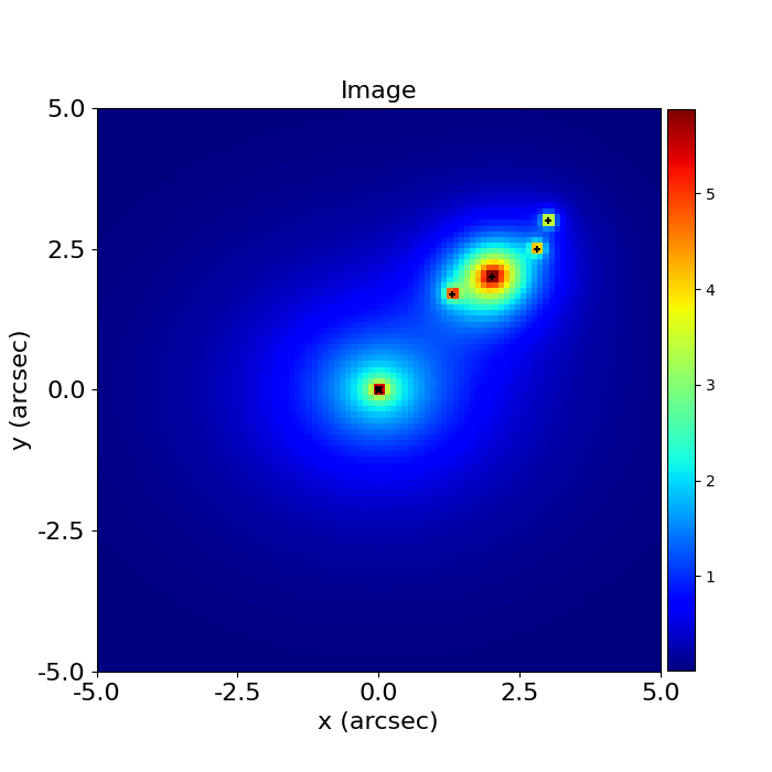
To finish, lets create a Plane with 2 merging galaxies, where the second galaxy has multiple star forming clumps.
galaxy_0 = ag.Galaxy(
    redshift=0.5,
    bulge=ag.lmp.Sersic(
        centre=(0.0, 0.0),
        ell_comps=(0.0, 0.05),
        intensity=0.5,
        effective_radius=0.3,
        sersic_index=3.5,
        mass_to_light_ratio=0.6,
    ),
    disk = ag.lmp.Exponential(
        centre=(0.0, 0.0),
        ell_comps=(0.0, 0.1),
        intensity=1.0,
        effective_radius=2.0,
        mass_to_light_ratio=0.2,
    ),
)

galaxy_1 = ag.Galaxy(
    redshift=1.0,
    bulge=ag.lp.Exponential(
        centre=(0.00, 0.00),
        ell_comps=(0.05, 0.05),
        intensity=1.2,
        effective_radius=0.1,
    ),
    clump_0=ag.lp.Sersic(centre=(1.0, 1.0), intensity=0.5, effective_radius=0.2),
    clump_1=ag.lp.Sersic(centre=(0.5, 0.8), intensity=0.5, effective_radius=0.2),
    clump_2=ag.lp.Sersic(centre=(-1.0, -0.7), intensity=0.5, effective_radius=0.2),
)

plane = ag.Plane(galaxies=[galaxy_0, galaxy_1])
This is what the merging galaxies look like:
Wrap Up#
If you are unfamiliar with galaxy morphology and not clear what the above quantities or plots mean, fear not, in chapter 1 of the HowToGalaxy lecture series we’ll take you through the above API in detail, whilst teaching you how to use PyAutoGalaxy at the same time! Checkout the tutorials section of the readthedocs!